

589


目次
モデル2学習
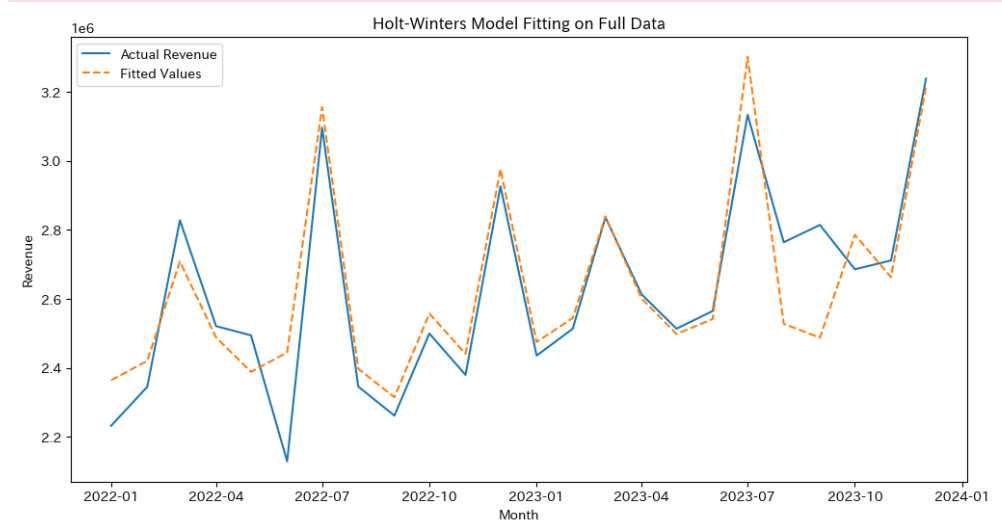
では次にトレンドを含めたモデルを作成していきます。
加法モデルです。
# 加法的トレンドと加法的季節性を持つモデルをフィットさせる
model_with_trend = ExponentialSmoothing(data['売上'],
                                        trend='add',
                                        seasonal='add',
                                        seasonal_periods=12).fit()

# モデルのフィット結果のプロット
fitted_values2 = model_with_trend.fittedvalues

plt.figure(figsize=(12, 6))
plt.plot(data['売上'], label='Actual Revenue')
plt.plot(fitted_values2, label='Fitted Values', linestyle='--')
plt.title('Holt-Winters Model Fitting on Full Data')
plt.xlabel('Month')
plt.ylabel('Revenue')
plt.legend()
plt.show()
あら、あまり先ほどと変わらない気がしますね(^▽^;)
params2 = model_with_trend.params

params_df2 = pd.DataFrame(list(params2.items()), columns=['Parameter', 'Value'])
params_df2 = params_df2[params_df2['Parameter'] != 'initial_seasons']
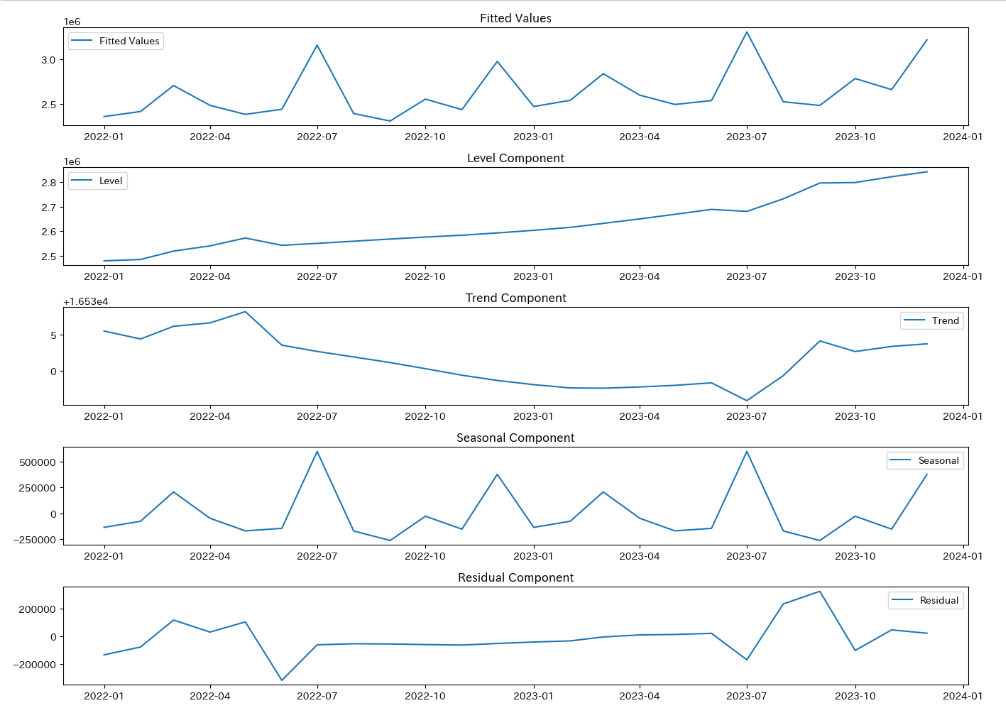
params_df2トレンド成分が追加されているのがわかると思います。
成分ごとにプロットしてみましょう。
# モデルの成分を抽出
fitted_values = model_with_trend.fittedvalues
level = model_with_trend.level
trend = model_with_trend.trend
seasonal =model_with_trend.season
resid = model_with_trend.resid

# 各成分のプロット
plt.figure(figsize=(14, 10))

plt.subplot(511)
plt.plot(fitted_values, label='Fitted Values')
plt.title('Fitted Values')
plt.legend()

plt.subplot(512)
plt.plot(level, label='Level')
plt.title('Level Component')
plt.legend()

plt.subplot(513)
plt.plot(trend, label='Trend')
plt.title('Trend Component')
plt.legend()

plt.subplot(514)
plt.plot(seasonal, label='Seasonal')
plt.title('Seasonal Component')
plt.legend()

plt.subplot(515)
plt.plot(resid, label='Residual')
plt.title('Residual Component')
plt.legend()

plt.tight_layout()
plt.show()
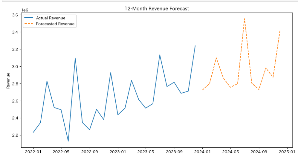
モデル2で予測
# 次の12ヶ月の売上を予測
forecast2_next_12 = model_with_trend.forecast(12)

# 予測結果のプロット
plt.figure(figsize=(12, 6))
plt.plot(data['売上'], label='Actual Revenue')
plt.plot(forecast2_next_12, label='Forecasted Revenue', linestyle='--')
plt.title('12-Month Revenue Forecast')
plt.xlabel('Month')
plt.ylabel('Revenue')
plt.legend()
plt.show()
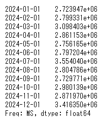
forecast2_next_12トレンド成分が入ったことによって予測が少し上向きになりました。
先ほどの予測と比較してみると...
(モデル1予測再掲)
後半に連れて上昇しているのがわかりますね!
まとめ
今回は、ホルトウィンターズ法で、トレンドなしとトレンドありの2つのモデルを実行しました。
データが少ないこともあり残差が残ってしまっている部分もありましたが、思いのほかいい感じに予測できたのではないかと思います。
もう少しデータがあればトレーニングセットとテストセットに分けて検証したいところでしたが、中小企業のデータはそんなにたくさんあるわけではないことが多く、その中で意思決定に寄与する最大限の分析をしていかなければなりません。
今回のホルトウィンターズ法が最善というわけではないと思いますので、実務ではもっといろいろ試してみる必要があります。
では♪
参考書籍
基礎からわかる時系列分析―Rで実践するカルマンフィルタ・MCMC・粒子フィルタ― Data Science Library
萩原 淳一郎 (著), 瓜生 真也 (著), 牧山 幸史 (著), 石田 基広 (監修)
時系列解析 自己回帰型モデル・状態空間モデル・異常検知 Advanced Python 1
島田 直希 (著)